Configure waste water events
Any referenced datasets can be downloaded from "Module downloads" in the module overview.
Step-by-step guide
In InfoWorks ICM, use waste water and trade waste events to model pollution.
- Waste water events describe the daily pattern of domestic waste from one or more subcatchment populations.
- Trade waste events describe the daily pattern of waste from industrial sources.
Each event can contain one or more profiles that describe the waste for subcatchments, and both types of profiles are edited similarly using the Profile Editor.
This example illustrates how pollution is modeled with a waste water event using a simple three-pipe model with one subcatchment.
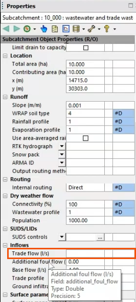
- Open the Properties for the subcatchment to view some important values: the Population value is set to 1000 and the Base flow is 4 liters per second.
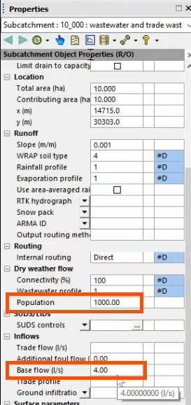
Note that base flow is clean, without pollution, and will dilute the population flow.
A waste water event applies the amount of pollution from each person. In this example, a waste water event has been completed and contains one profile for a single subcatchment.
To review the configuration:
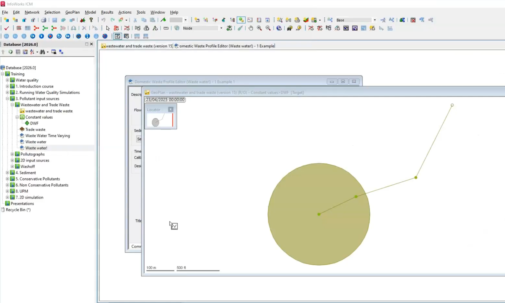
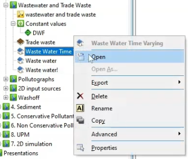
- From the Explorer window, right-click the Waste water event and select Open.
In the Domestic Waste Profile Editor, two sets of parameters can be edited for each profile.
- Fixed parameters, including the per capita flow and water quality aspects, are located on the Common tab.
- Time-dependent multipliers are located on the Profile tab.
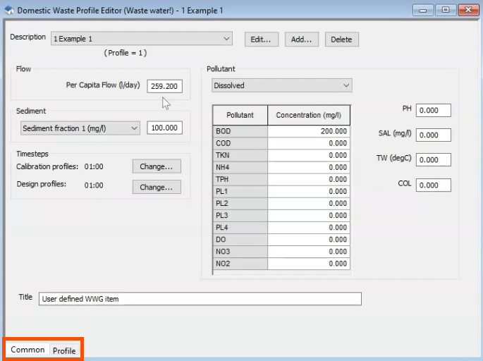
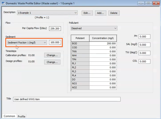
Fixed parameters:
For this example, the Per Capita Flow is set to 259.2 liters per person per day. This specific number was chosen to generate a whole number for population flow, but you will enter a more realistic flow.
When per capita flow is multiplied by the population, and the result is converted to liters per second, this equates to almost exactly 3 liters per second (l/s) of population flow.
Population Flow = Per Capita Flow (259.2 l/d) x Population (1000)
= 25.92 cubic meters per day
= approximately 3 liters per second (l/s)
Again, this number simplifies subsequent calculations using fixed parameters.
- To calculate the total inflow, add the 3 l/s of polluted flow from the population to the clean Base flow identified in the subcatchment Properties.
Flow = Population Flow (3 l/s) + Base Flow (4 l/s) = 7 l/s
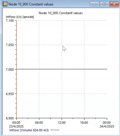
To review these results, graph the inflow:
- From the Results toolbar, click Graph.
- In the GeoPlan, select the inflow node of the subcatchment.
- In the Graph dialog, select Inflow (l/s).
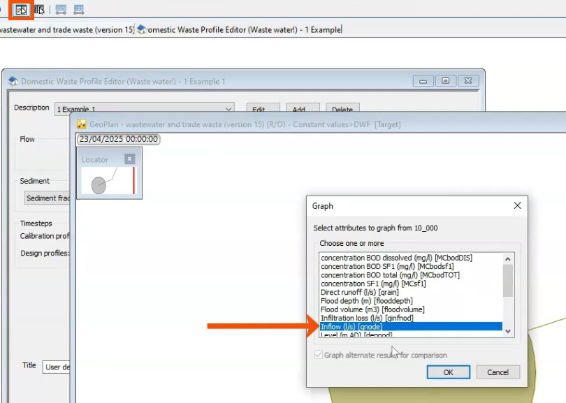
- Click OK.
The resulting graph shows a constant 7 l/s, which matches the calculation.
- Open the Profile Editor again to review the water quality aspects, noting that Sediment Fraction 1 (SF1) is set to 100 milligrams per liter.
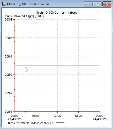
- Multiply this SF1 value by the population flow to calculate the mass inflow of Sediment fraction 1 (MfSF1).
MfSF1 = 3 l/s x 100 mg/l = 0.3 g/s
- Graph the mass inflow SF1 (g/s).
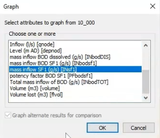
The graph displays the same result, 0.3 grams per second (g/s).
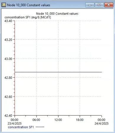
- To find the concentration of Sediment Fraction 1 (CnSF1), divide the mass inflow by the total inflow.
CnSF1 = Mass Flow (0.3 g/s) / Flow (7 l/s) = 42.85 mg/l
- Graph the concentration SF1 (mg/l) to see that the results match.
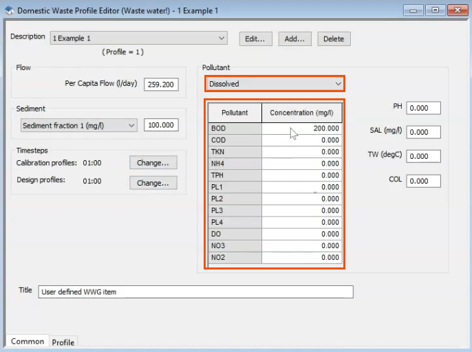
Dissolved constituents can also be assigned.
Back in the Profile Editor, note that with the Pollutant drop-down set to Dissolved, the table shows each pollutant and its dissolved concentration. In this case, the biochemical oxygen demand (BOD) is set to 200 milligrams per liter.
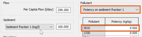
This drop-down can also be used to assign potencies for either sediment fraction.
- In the drop-down, select Potency on sediment fraction 1. In this case, a potency of 0.5 kg/kg is assigned for BOD.
- To calculate the mass inflow of BOD dissolved (MfBODd), multiply the population flow by the pollutant concentration of 200 mg/l.
MfBODd = 3 l/s x 200 mg/l = 0.6 g/s
- To calculate the mass inflow of the attached constituent (MfBOD1), multiply the mass inflow of SF1 by the potency factor of 0.5.
MfBOD1 = MfSF1 x PFBOD1 = 0.3 g/s x 0.5 = 0.15 g/s
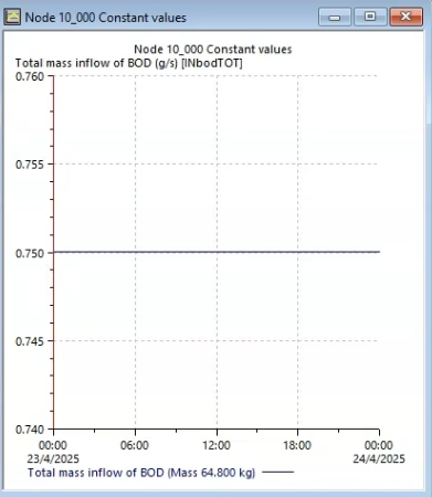
- Add the mass inflow of the dissolved and attached pollutant together to find the total mass inflow of BOD (MFBODt).
MFBODt = MfBODd + MfBOD1 = 0.6 g/s + 0.15 g/s = 0.75 g/s
- Graph the Total mass inflow of BOD (g/s) to achieve the same result.
Time-dependent parameters:
The other set of parameters that can be edited for each profile is time-dependent multipliers.
- Used to create a time-varying profile from the fixed parameters.
- Different pollutant loads can be assigned at different times of day, different days of the week, or even different months of the year.
In this example, a time-varying event has already been created.
- Right-click the Waste Water Time Varying event and select Open.
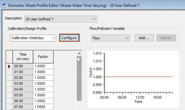
- In the Profile Editor, select the Profile tab.
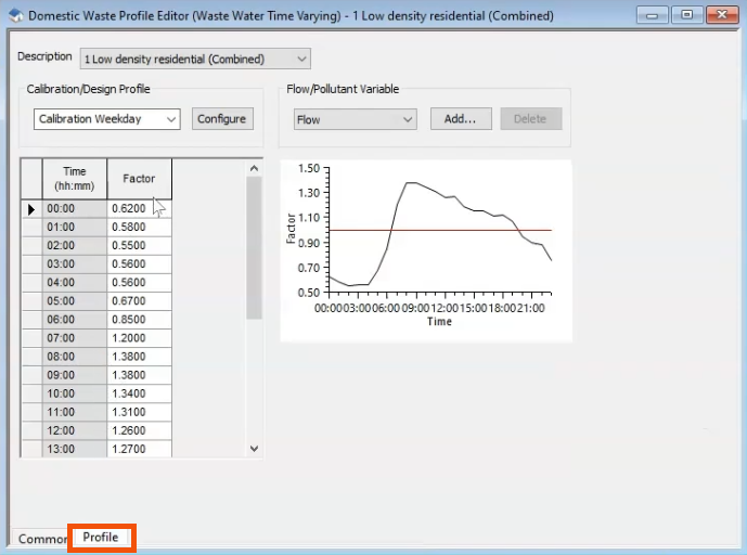
There are 24 different factors to consider that apply to nominal flow or pollutant values. It is critical to confirm that the factors add up to 24, to help ensure that flow and sediment values assigned on the Common tab are accurately applied. If the factors do not average to 1, flow and sediment values will be adjusted.
- Expand the Calibration/Design Profile drop-down and choose:
- Calibration Weekday to run weekday simulations.
- Calibration Weekend to run weekend simulations.
- Calibration Monthly for different monthly multipliers used with varying populations throughout the year, such as student or tourist populations.
- Design to define profiles for design storms.
- Use the Flow/Pollutant Variable drop-down to vary the concentration of pollutants. Here, select General Pollutant.
In the updated graph, at 9:00 AM, the flow is greater and more polluted due to higher concentrations of general pollutants.
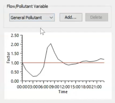
With General Pollutant selected, all pollutants act the same. However, pollutants can be added that will act differently.
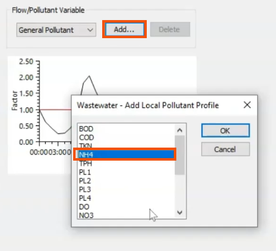
- Click Add.
- Select a pollutant, such as NH4.
- Click OK.
- Use the table to define the pollutant profile.
Alternatively, configure calibration profiles to calculate different values on different days of the week.
- Click Configure.
- In the Configure Calibration Profiles dialog, select the required days of the week for each profile.
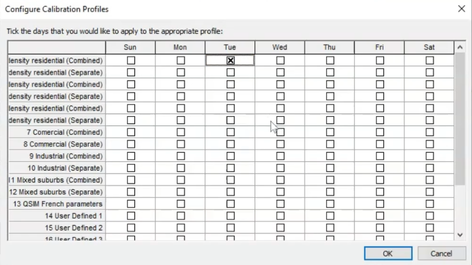
- Click OK.
The calibration profile for each day selected will be available for editing in the drop-down, and the selected profiles will be applied to the flow and pollutant variables of the event profile.
Trade events act similarly to waste water events except:
- A trade event describes flow from a single source instead of per capita flow.
- In the subcatchment properties, a Trade flow value is entered instead of multiplying the population by the flow per person.
- Open the Profile Editor for a Trade waste event to see that the per capita flow field is replaced by the Flow Scaling Factor.
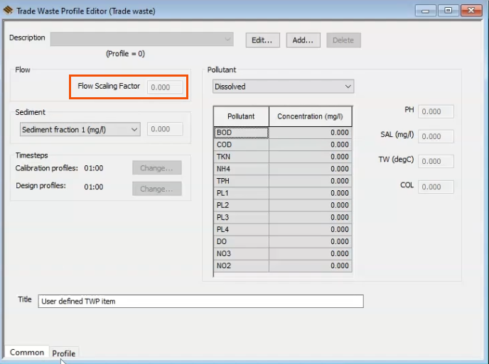
The process of defining profiles and setting up concentrations is identical to waste water events.