Simulate pollutant washoff
Any referenced datasets can be downloaded from "Module downloads" in the module overview.
Simulate pollutant washoff
Step-by-step guide
In ICM, water quality simulations can model sediment buildup and the movement of sediment and determinants in a drainage system during rainfall.
Pollutant washoff refers to the pollutants that build up on a catchment surface and are washed into a sewer system by rainfall.
The volume of pollutants on the catchment surface and the speed with which they are washed into the sewer can be controlled in the water quality calculations during the simulation.
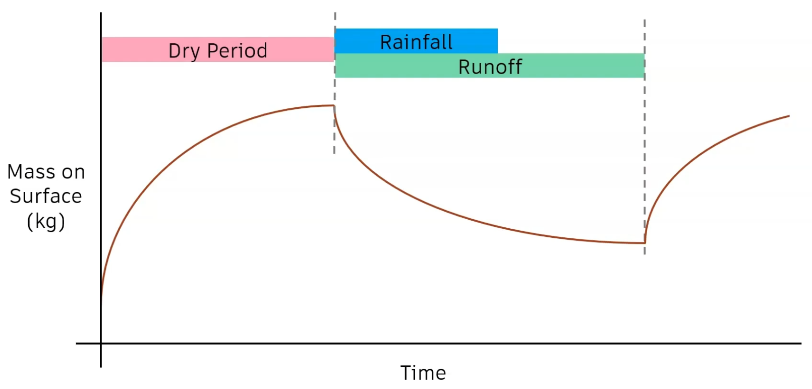
The graph below demonstrates the mass of pollutant on the catchment surface as a function of time:
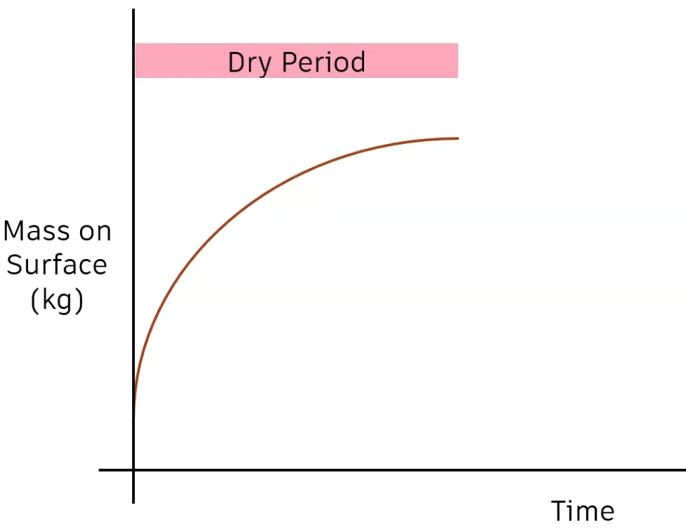
- The buildup time is a period of dry weather when surface sediment builds up.
- The rate of increase decreases with time.
- Generally, the buildup starts from zero; however, a specific mass of pollutant can be defined to start.
There are different methods to define the buildup within a simulation.
In a continuous simulation with periods of rainfall and dry weather, the process is applied automatically, with buildup occurring during dry periods, and washoff during wet periods.
In a simulation with a single event or several rainfall events, a consistent buildup time can be specified in the Run schedule QM Parameters.
- With a network model already created and opened, open the Run dialog.
- Click QM parameters.
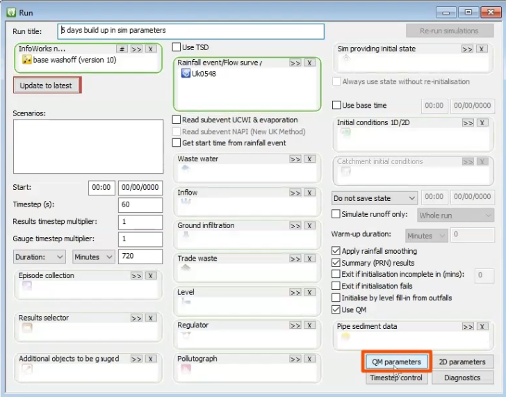
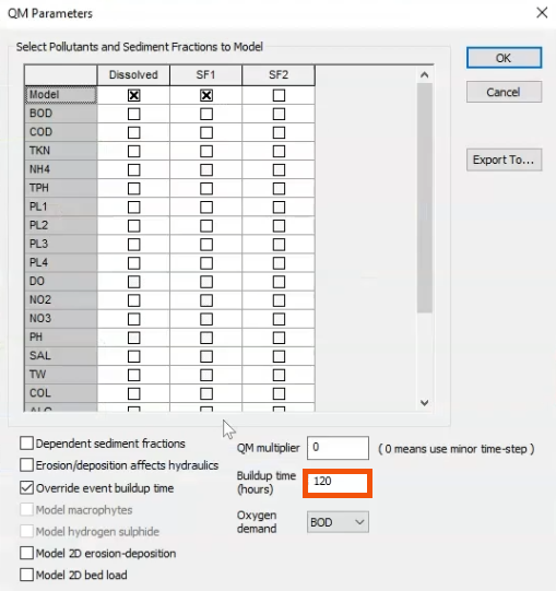
- In the QM Parameters dialog, specify the Buildup time in hours.
In a time series event, define individual buildup times as part of each rainfall event.
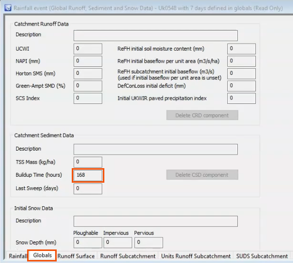
- From the Explorer window, within a model group, right-click an existing rainfall event and select Open.
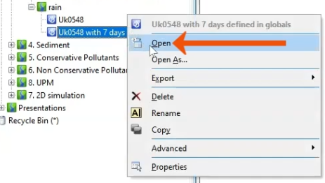
- From the Rainfall event dialog, open the Globals tab.
- Under the Catchment Sediment Data group, enter the Buildup Time in hours.
Review the impact of buildup time by comparing simulations with:
- Zero buildup time.
- Five days of dry weather calculated in the simulation parameters' buildup time.
- Seven days of dry weather applied in the rainfall event itself.
To graph the first simulation:
- From the Explorer, click and drag base run into the graphics window.
- Select Results > Graph reports > Simulation report.
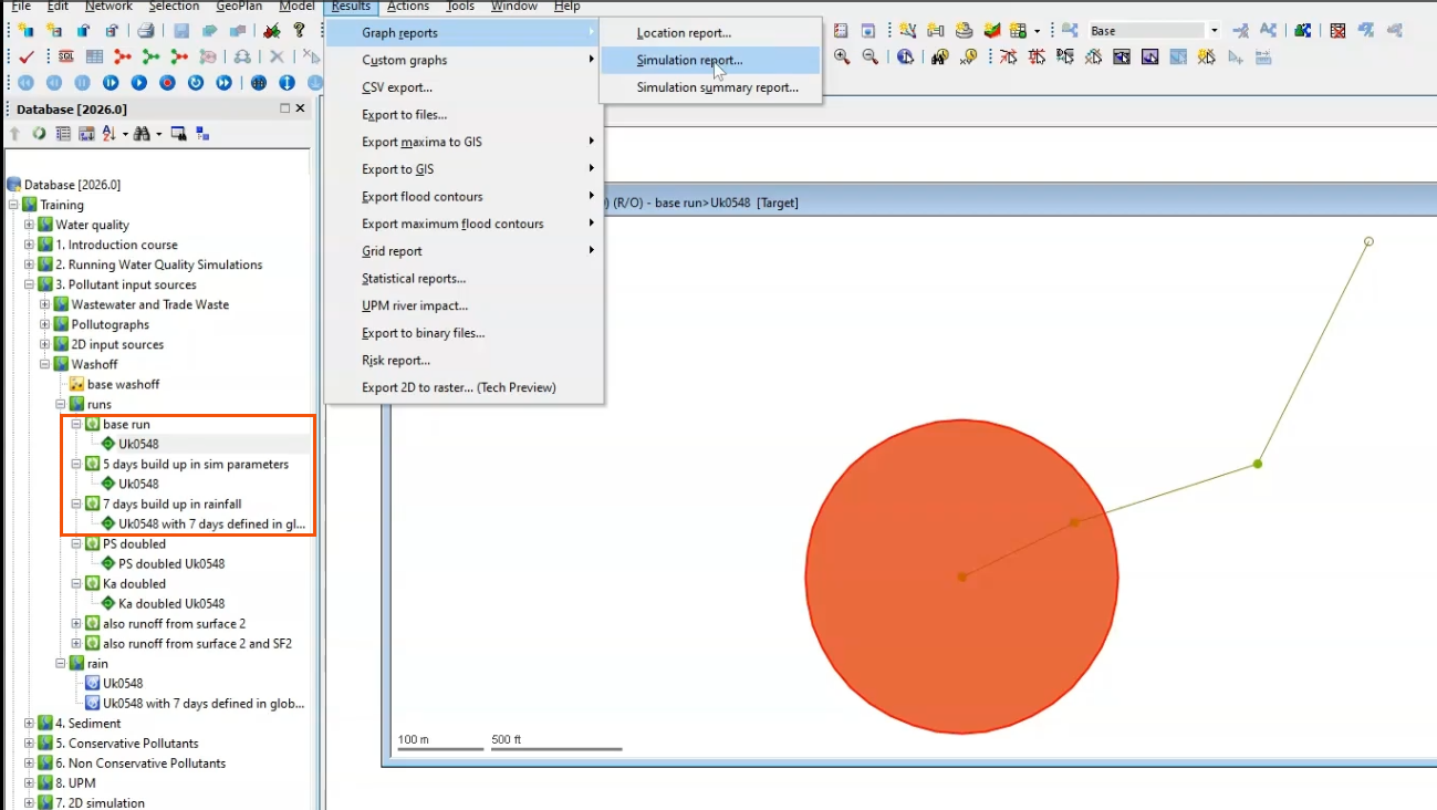
The Simulations dialog opens.
- Drag 5 days build up in sim parameters into the Simulations dialog.
- Drag 7 days build up in rainfall into the dialog.
- Click Produce Graphs.
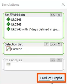
- In the Parameter Selection dialog, under Parameters, select Washoff SF1.
- Click OK.
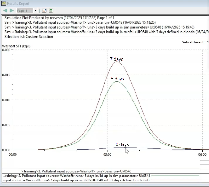
- In the graph, review how buildup time affects washoff.
- With 0 days of buildup, there is almost no washoff.
- After 5 days of buildup, there is a significant increase in washoff.
- After 7 days of buildup, the washoff increases slightly more.
Following buildup, or the dry period, rainfall causes runoff and reduces the mass on the catchment surface due to washoff.
In a continuous simulation, runoff is followed by accumulation again.
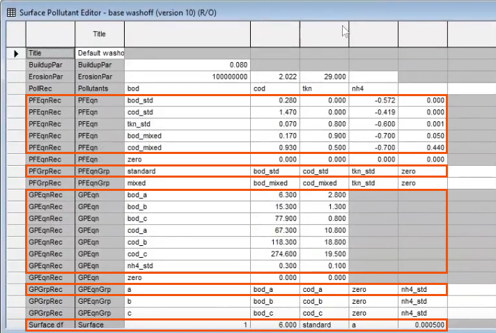
Runoff and washoff parameters can be controlled in the Surface Pollutant Editor. They are used to calculate pollutant buildup and washoff on catchment surfaces and in gully pots.
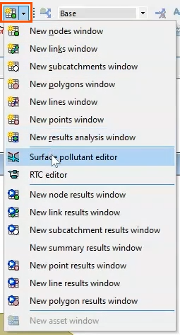
- To access the editor, from the Windows toolbar, expand the Grid Windows drop-down and select Surface pollutant editor.
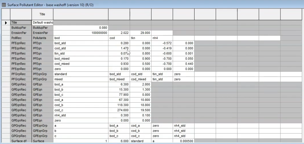
The editor displays a series of records that can be used to define pollution indices, global buildup and erosion characteristics for sediment, or parameters for sediment fractions.
Refer to the Autodesk InfoWorks ICM Help topic, Surface Pollutant Editor, for more information on each record type and the fields that they contain.
In the image below, the equations used by the model are overlaid on the editor, with color-coded arrows connecting parameters and their corresponding values.
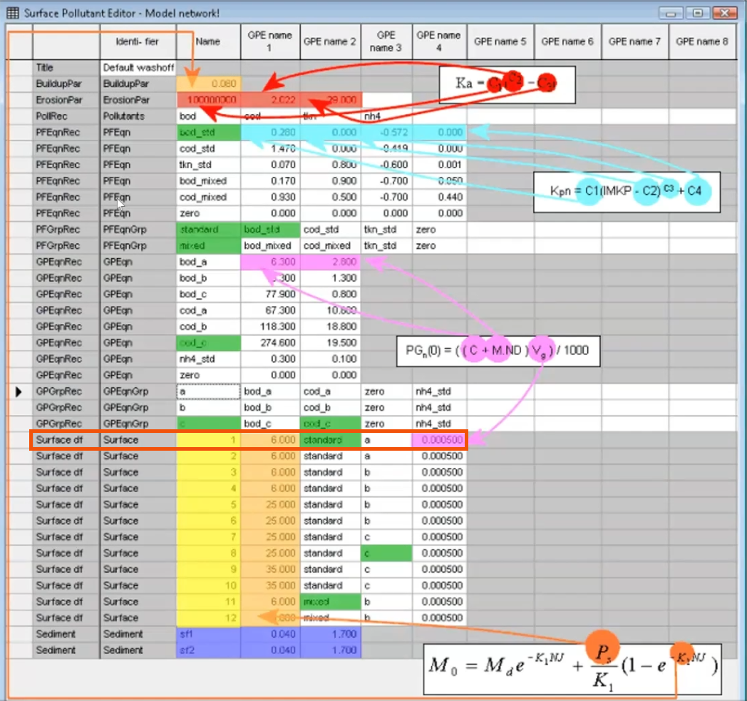
The records listed in the editor correspond to specific equations.
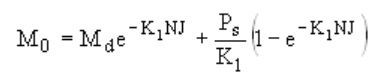
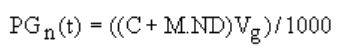
- Buildup Parameters record (BuildupPar): Used in the surface buildup equation to calculate the mass of sediment buildup on the catchment surface. To increase the buildup rate, increase the dry period or the surface factor, PS. Note that only SF1 is used for washoff; it is not possible to use SF2.
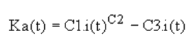
- Erosion Parameters Record (ErosionPar): Used in the rainfall erosion coefficient equation to calculate sediment deposits left on the catchment surface that are washed off. This defines the speed of washoff as a function of rainfall. For example, an increase in parameter C1 increases washoff for that rainfall event.
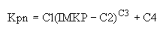
- Potency Factor Equation record (PFEqnRec): Used to determine the potency factors (Kpn) of pollutants, which are used to relate the surface mass of the sediment to the surface mass of the attached pollutant.
- Gully Pot Buildup Equation record (GPEqnRec): Used to determine the buildup of dissolved pollutants in gully pots during the buildup period of the simulation and for each simulation timestep.
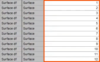
The Pollution Index is the water quality equivalent of a Runoff Surface that is associated with a subcatchment through the Land Use definition, with up to twelve surfaces.
To use the Land Use definition file, first, identify the index that is linked to the subcatchment.
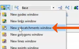
- With the base run open, from the Windows toolbar, in the Grid windows drop-down, select New subcatchments window.
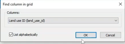
- In the Subcatchment grid, right-click any column header and select Find column.
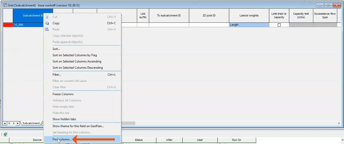
- In the Find column in grid dialog, select Land use ID.
- Click OK.
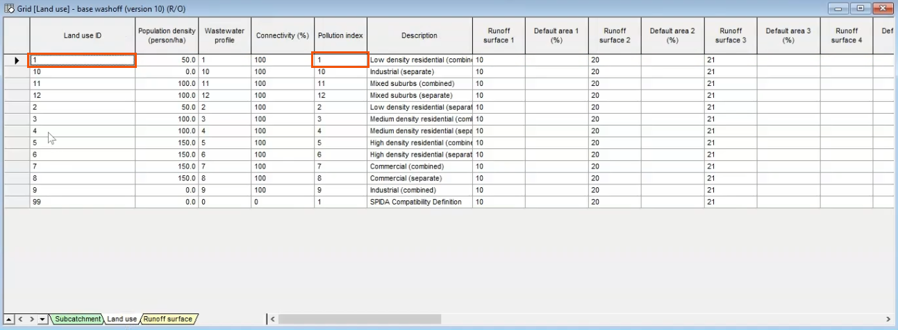
- In the Subcatchment Grid, in the highlighted Land use ID column, note the ID of 1.

- In the Grid, select the Land use tab, where anything in row 1 also applies to this subcatchment.
In this case, Land use ID 1 relates to Pollution Index 1.
- Return to the Surface Pollutant Editor and locate the subcatchment linked to Index 1.
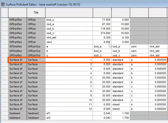
Several parameters apply to this subcatchment:
- The two numeric values represent terms in the buildup equation and the dissolved pollutants equation, respectively. If needed, refer back to the color-coded image to visualize these links.
- There are also two indices, “standard” and “a”, meaning that two further rows in this file apply.
- Locate the “standard” and “a” rows.
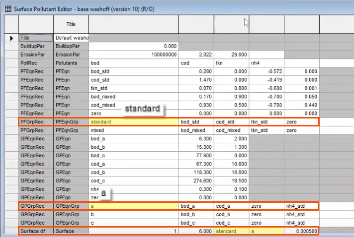
The “standard” and “a” rows include additional indices, including “bod_a” and “cod_a,” that define the attached pollutants and the dissolved pollutants.
- Again, identify all of the applicable rows.
While this file may look complicated, it is only because of the complex way in which it is linked together. To manipulate the equations, the important thing is to identify the pollution index for each subcatchment and the subsequent parameters that it is linked to.
Next, use the buildup equation and the washoff equation to compare three scenarios:
- A base run.
- PS doubled, with the PS value doubled in the buildup equation to result in more sediment on the catchment surface, and therefore, more washoff.
- Ka doubled, with the C1 parameter doubled in the washoff equation to result in a faster washoff.
- Open the base run.
- With the subcatchment selected in the GeoPlan, select Results > Graph reports > Simulation report.
- Drag the second and third simulations into the Simulations dialog.
- Click Produce Graphs.
- Select Washoff SF1.
- Click OK to review the results.
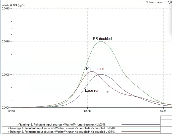
For PS doubled, since there was a significant increase in the amount of sediment accumulating on the catchment surface, there is an increased volume of washoff.
Ka doubled, which had an increase in washoff rate only, shows the same volume of sediment entering the sewerage system as the base run; but it is entering faster, as a function of rainfall.